A couple of weeks ago I ran into a problem where I needed to create some spatially correlated data for a project and I realized that I didn’t know the first thing about how to go about doing it. I was lucky to find that the paper that I was trying to replicate did a great job of detailing their methods in such a way that I was able to create some spatial data of my own. The idea is that you need to create a covariance matrix of the relationships of your data to pull form a multivariate random normal distribution.
is just the scalar mean and can be set to any real number but defining a sensible covariance matrix was originally difficult. The way that Riebler et al. did it was by using a matrix Q
where is the number of neighbors a location has and means that the two locations are adjacent. Im used to working with spatial polygons data frames in R and found that its pretty easy to create this matrix with the right packages. Here’s an example with US state shape file.
library(sp)
library(surveillance)
library(spdep)
library(MASS)

# load in some USA data to work with
load(url("http://biogeo.ucdavis.edu/data/gadm2/R/USA_adm2.RData"))
cont_usa_locs <- c("Texas", "Louisiana")

# spatial polygons data frame to simulate from
cont_usa <- gadm[(gadm@data$NAME_1 %in% cont_usa_locs),]
cont_usa$ID <- 1:length(cont_usa)

# adjacency matrix for spatial data 1's if adjacent 0 otherwise
adjmat <- poly2adjmat(cont_usa)

# Create Q from an adjacency matrix
n_delta_i <- rowSums(adjmat)
Q <- adjmat * -1
diag(Q) <- n_delta_i
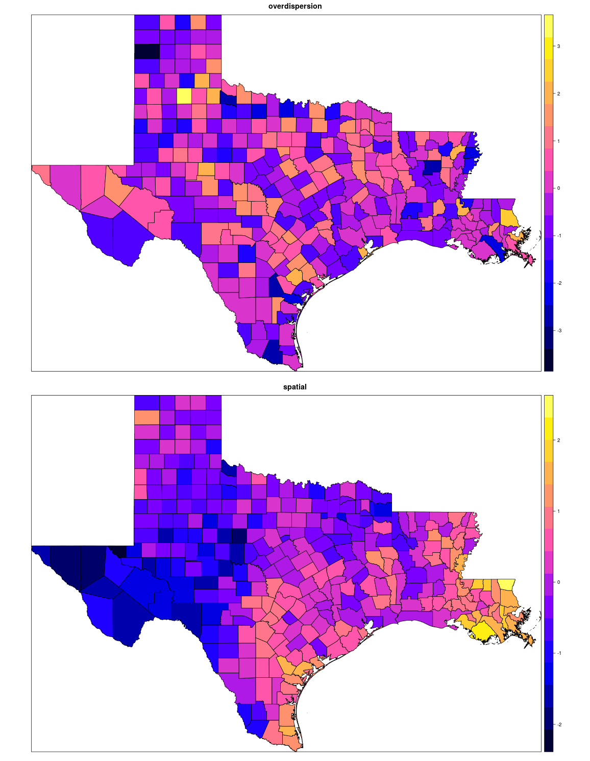
Using the inverse of Q as the covariance matrix creates a smooth spatial dispersion, that you can see below, when compared to just simple dispersion at random. A more complete example can be found here.
